Evaluating Power-Demand Reduction With VFD-Controlled Systems

Pressure losses, including friction and local resistance losses, are variable and depend on the velocity of the fluid travelling through a pipe or duct, while static-pressure losses (i.e., vertical elevation loss to lift fluid to a point of utilization and/or minimum required pressure differential at a terminal unit, etc.) could be assumed constant and independent of fluid velocity. We combined friction and local resistance pressure losses into a single category: dynamic pressure losses. This assumption is convenient for the analysis applied in Figure 1.

Figure 1 demonstrates how the ratio between the relative (dimensionless) design dynamic and static-pressure loss impacts overall relative pressure drop in a closed-loop system, which, in turn, influences system power demand. For convenience, we assumed the curve of the system in Figure 1A (for the quadratic relation between pressure drop and flow rate) would go through the origin. The graphs in Figure 1 were built on the assumption the VFD would have a turndown ratio (TDR) of 10 to 1, which is typical of VFDs. This was done by varying the speed of the electrical motor via the changed electrical-power frequency from 60 Hz to 6 Hz. This meant the ratio of current flow rate to design flow rate (the relative flow-rate ratio [RFR]) would vary from 1.0 (design) to 0.1 (minimum). We further assumed the installed horsepower of the electrical motor and VFD would match the system design load. System relative pressure losses (∆P_SYS) were calculated from the following equations:

∆P_{SYS DES} = SORPL_DES = (DRPL_DES + SRPL_DES) = 1.0                                                   (1)

∆P_{SYS CUR} = SORPL_CUR = (DRPL_CUR + SRPL_CUR) ÷ SORPL_DES                                     (2)

DRPL_CUR = DRPL_DES × RFRⁿ⁼²                                                                                         (3)

SRPL_CUR = SRPL_DES × RFRⁿ⁼⁰                                                                                          (4)

where:

∆P_{SYS DES} = system relative pressure losses at design conditions

SORPL_DES = system overall relative pressure losses at design conditions

DRPL_DES = system relative dynamic pressure losses at design conditions

SRPL_DES = system relative static-pressure losses at design conditions

∆P_{SYS CUR} = system relative pressure losses at current conditions

SORPL_CUR = system overall relative pressure losses at current conditions

DRPL_CUR = system relative dynamic pressure losses at current conditions

SRPL_CUR = system relative static-pressure losses at current conditions

ⁿ = exponential index parameter varying from 0 for relative static system pressure losses to 2 for relative dynamic system pressure losses

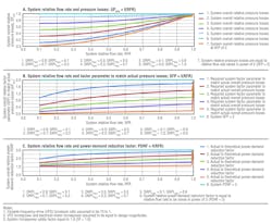
Although dynamic pressure losses follow relative changes in flow rate elevated to the power of 2, system overall pressure losses consisting of both dynamic- and static-pressure components do not. There are, however, two exceptions: the theoretical cases of systems with no dynamic pressure losses (SRPL_DES = 1.0; DRPL_DES = 0.0) or no static-pressure losses (DRPL_DES = 1.0; SRPL_DES = 0.0). These cases are shown by Line 6 and Curve 7, respectively, in Figure 1A. The rest of the curves between Line 6 and Curve 7 are related to relative design dynamic pressure losses (DRPL_DES) varying from 0.9 to 0.1 and relative design static-pressure losses (SRPL_DES) varying from 0.1 to 0.9. Figure 1A indicates the system overall relative pressure drop (∆P_SYS) could deviate significantly from the theoretical assumptions. For instance, for the system with DRPL_DES of 0.9, ∆P_SYS varies from 1 to 0.1 when RFR varies from 1 to 0.1. On the other hand, for the system with DRPL_DES of 0.5, ∆P_SYS varies only from 1 to 0.5 when RFR varies from 1 to 0.1.

In the following analysis, we introduced system factor parameter (SFP), which indicates overall functional dependency between system pressure loss and flow rate. The following equation was utilized:

∆P_SYS = SORPL_CUR ÷ SORPL_DES = RFR^SFP                                                                     (5)

Equation 5 allows the magnitude of SFP for various combinations of ∆P_SYS and RFR, which are shown in Figure 1A, to be found. Figure 1B demonstrates how the actual value of SFP in Equation 5 depends on the system-pressure-drop-distribution pattern between design dynamic and static components of the pressure loss described earlier. SFP represents the average weighted magnitude of the exponent in the equation, which should be applied to relative flow rate to match system relative pressure drop. The top straight line in Figure 1B (No. 6) represents the theoretical case in which system pressure losses are caused by dynamic losses only, which is equivalent to an exponent value of 2 (SFP = 2). This straight line correlates to Line 7 in Figure 1A. The rest of the curves in Figure 1B represent various combinations of system dynamic and static losses and are correlated to curves 2 through 6 in Figure 1A. The Figure 1B curves indicate SFP values could vary substantially to match system relative pressure drop and could be well below the theoretical value of 2, which typically is utilized in engineering designs with VFD applications.

Figure 1B also demonstrates the SFP does not remain constant and varies depending on the ratio of relative design dynamic-pressure losses to static-pressure losses, as well as RFR. Figure 1B shows the usual control strategy of maintaining design pressure differential at an RFR of 1.0 could be improved by resetting the controlled pressure differential as a function of RFR.

Accepting the theoretical case as the design baseline might lead, as shown in figures 1B and 1C, to overestimating magnitudes of potential energy savings associated with VFD applications.

The field areas between Line 6 and the five other curves in Figure 1B show the potential reduction in system relative pressure losses. The greater the magnitude of design system relative static-pressure losses, the larger the field areas.

Similarly, Figure 1C shows system overall relative power-demand reduction ratio (PDRR) as compared with the theoretical value of 3. System PDRR will be in direct proportion to the variation in system relative pressure differential (Figure 1B) and RFR. Line 6 in Figure 1C represents the theoretical PDRR of 3 for the case in which all pressure losses are caused by dynamic losses (correlated with Curve 7 and Line 6 in Figure 1A and 1B, respectively). The other five curves in Figure 1C outline PDRR for various distribution patterns between relative design dynamic and static-pressure losses. Thus, the field areas between Line 6 and each of the other curves represent the reduction in available power-demand savings for various operational loads, which correlate with respective RFR values. Once again, the higher the magnitude of system relative static-pressure losses, the larger the field areas between a theoretical value of 3 and actual PDRR.

Assuming the efficiency of an electrical motor and pump or fan remains constant, the calculation of system relative power demand (RPD) could be simplified. When combined with ∆P_SYS from Equation 5, the magnitude of RPD could be presented as follows:

RPD = ∆P_SYS × RFR^1.0 = RFR^SFP × RFR^1.0 = RFR^PDRF                                                   (6)

where:

PDRF = SFP + 1 = system power-demand reduction factor

Equation 6 allows the magnitudes of PDRF (shown in Figure 1C) for various combinations of ∆P_SYS (shown in Figure 1A) and RFR to be found.

For the system with dynamic pressure losses only, the theoretical PDRF will be 3. For the systems having both dynamic and static-pressure losses, the PDRF will be less than 3.

PDRF could vary from 2.8 at an RFR of 0.99 for a DRPL_DES of 0.9 (Curve 1 in Figure 1C) to 1.96 at an RFR of 0.1. Thus, for this system, the PDRF magnitude compared with its theoretical value of 3 could be overestimated by as much as 43.3 percent on average over the course of a year, assuming equal-weight-time-distribution occurrences at various loads from an RFR of 1.0 to an RFR of 0.1. Utilizing the same approach for the systems with a DRPL_DES of 0.7 (Curve 2 in Figure 1C) and 0.5 (Curve 3 in Figure 1C), the reduction in potential annual power-demand savings as compared with the theoretical case could be as high as 130 percent and 216 percent, respectively.

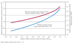
Figure 2 shows the variation in relative average annual SFP and PDRF as a function of DRPL_DES magnitude. SFP varies from 2 (theoretical case) at a DRPL_DES of 1.0 to 0.3 at a DRPL_DES of 0.1. This again demonstrates how significant deviation from a theoretical case could be. Figure 2 also shows that, for the considered conditions, PDRF deviates quite noticeably from its theoretical value of 3 at a DRPL_DES of 1.0 to 1.3 at a DRPL_DES of 0.1.

This analysis was conducted for the conditions under which the electrical motor and VFD were sized to match system design load. However, often, an electrical motor and a VFD are sized with safety factors (or load factors), especially for industrial and commercial applications.

Safety factors also are applied to compensate for VFD-capacity derating conditions precipitated by a deviation from given optimal switching frequency for a drive, VFD-enclosure cooling air temperature, etc. In these instances, derating conditions might reduce a drive’s output current, which would require utilization of oversized drives. Designers quite often oversize electrical-motor horsepower to increase system reliability and redundancy. Typically, system safety factors vary from 1.0 to about 2.0.

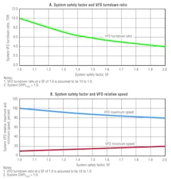
Figure 3 shows the correlation between system VFD TDR (Figure 3A) and VFD maximum and minimum speed (Figure 3B) for five safety factors. For example, at a TDR of 10 to 1 (safety factor of 1.0), the system VFD maximum and minimum speed will be 100 percent and 10 percent, respectively. For instance, if the safety factor for both an electrical motor and a VFD is 1.33 when DRPL_DES is 1.0, then the system design load will be satisfied when the electrical motor is running at 91 percent, instead of 100 percent, of its maximum speed. Furthermore, under this scenario, the system VFD TDR of 10 to 1 will be reduced to 6.8 to 1, or lowered by 32 percent.

If we assume a safety factor of 2.0 for an electrical motor and a VFD, then the design load will be satisfied when the electrical motor runs near 80 percent of its maximum speed. For these conditions, the system VFD TDR of 10 to 1 will be reduced to 4 to 1, or lowered by 60 percent.

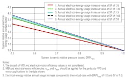
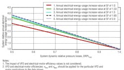
Figure 4 demonstrates (for steady-state operational conditions) the impact of system relative dynamic-pressure losses on magnitude of potential overestimation of annual electrical-energy savings. The assumption for the baseline conditions (Line 1) was that, at a DRPL_DES of 1.0, the same magnitude of safety factor (1.0) will be applied for the electrical motor and VFD. Figure 4 indicates the application of the safety factor could decrease potential annual power-demand reduction and electrical-energy savings compared with the theoretical case. The reduction in power demand and energy savings depends on the rate of increase of safety factor. This savings reduction will occur for safety-factor values ranging from 1.33 to 1.65. Above this magnitude, the rate of reduction in savings will remain constant. This happens because at this point, any further increase in safety factor will reduce potential rate of increase of electrical savings at lower VFD speeds because of reduced VFD TDR.

The impact of safety factor still could be quite substantial. For instance, Figure 4 depicts the increase in annual electrical-energy use with a DRPL_DES of 0.5 and a safety factor of 2.0 could be 22.5 percent compared with the system with a safety factor of 1.0. However, this impact will diminish at higher values of DRPL_DES.

Figure 4 could be used to evaluate magnitude of relative annual energy savings for VFD applications compared with the theoretical baseline case. For instance, for the system with a DRPL_DES of 1.0 and a safety factor of 1.0, the energy savings at the average relative annual load of 0.55 (i.e., ∑[1 + 0.9 + 0.8 + 0.7 + 0.6 + 0.5 + 0.4 + 0.3 + 0.2 + 0.1] ÷ 10) will yield a reduction factor of 6 (i.e., 1/[0.55³]) as compared with the system with no VFD control. However, for the system with a DRPL_DES of 0.7 and a safety factor of 1.0, the energy savings will produce the diminished reduction factor of 2.6 (i.e., 6 ÷ 2.3) because of the increase in relative annual electrical-energy use (Figure 4). Furthermore, if in addition to the latter conditions, the system safety factor will increase to 1.65, then the annual energy savings will yield the lower reduction factor of 2.2 (i.e., 6 ÷ 2.7) compared with the system with no VFD control (Figure 4). Thus, the theoretical annual electrical-energy savings will exceed their actual value by the factor of 2.7 (i.e., 6 ÷ 2.2).

Because VFD efficiency losses vary approximately in direct proportion to VFD horsepower load, any increase in electrical load for the system with a DRPL_DES of less than 1.0 and a safety factor greater than 1.0 might lead to reduced VFD efficiency and increased power demand at off-design operational conditions. This should be considered during system design.

System With VFD↔VFD Bypass Power-Demand Control for Electrical Motors

It is well known a VFD will increase system power demand when an electrical motor is running at or near maximum speed. Consideration of actual system design DRPL and SRPL values and VFD and electrical-motor safety factors may lead to reduced overall VFD efficiency and, thus, increased system power demand. An increase in system power demand, which is most critical during design and near-design operational conditions, can be offset with an advanced control system that allows realization of an optimal control strategy for switchover from VFD to VFD-bypass and from VFD-bypass to VFD modes of operation.¹ This control system can be employed for new applications as well as for retrofits to optimize electrical-motor power demand. An electrical utility experiencing a shortage in (kilowatt) capacity during peak-demand hours could use it to reduce system cumulative power demand, rather than add power-plant capacity.

At certain operational conditions, the power demand of an electrical motor running at variable speed and frequency will be equal to the power demand of the motor running at constant speed and frequency (i.e., line-voltage operation during VFD bypass mode). The operational point for switchover from VFD bypass to VFD control is defined by the conditions under which system power demand with VFD control becomes lower than system power demand at constant speed and frequency. Switchover can be implemented locally, at the end-use location, or remotely, from the site of the electrical utility.

Conclusions

Takeaways from this analysis are:

• Pressure loss in any system is defined by variable dynamic-pressure and constant static-pressure components.
• Common engineering evaluation of potential annual power-demand reduction and electrical-energy savings with VFDs typically is based on the assumption that hydraulic pressure drop in a system is caused by dynamic losses only. Therefore, system relative pressure loss and power-demand reduction follow relative flow-rate change, which is raised to the exponential indexes of 2 and 3, respectively. This could lead to a substantial overestimation of power-demand reduction and electrical-energy conservation associated with VFD control, increasing the payback period for a VFD system.
• The higher the design ratio of dynamic-pressure losses and lower the design ratio of static-pressure losses as compared with total system pressure losses, the greater the power-demand reduction and electrical-energy savings for VFD systems.
• Utilization of variable magnitudes of SFP and PDRF at a given relative flow rate to determine hydraulic pressure losses and power-demand changes during off-design conditions for various ratios of design dynamic- and static-pressure losses is suggested.
• Energy savings for systems with VFDs could be improved by applying variable pressure-differential-setpoint control instead of maintaining constant design magnitude of pressure differential.
• In addition to power-demand increase during design conditions, VFD application for electrical motors servicing systems with relative design dynamic-pressure losses less than 1.0 and safety factors higher than 1.0 might lead to increased power demand during off-design conditions. Power demand for systems with VFD control could be optimized by employing a switchover control strategy between VFD and VFD-bypass modes. This could reduce power demand for customers and electrical utilities during most critical operations at or near system electrical peak-power conditions.

Reference

1) Burd, A.L., & Burd, G.S. (2012). Optimized power demand control system for electrical motors. United States Patent US 8,143,819 B2. 8 claims, March 27, 2012.

Alexander L. Burd, PhD, PE, is president of, and Galina S. Burd, MS, is a project manager for, Advanced Research Technology, an engineering and research consulting firm with offices in Suffield, Conn., and Green Bay, Wis. Alexander ([email protected]) has 35 years of experience in the design, research, and optimization of HVAC and district energy systems, which includes publication of more than 35 research and technical papers in American and European journals, while Galina ([email protected]) has more than 25 years of design and research experience in the HVAC and architectural-engineering field and has co-authored many technical and research papers in American journals. Alexander and Galina have co-authored three U.S. patents related to energy conservation.

Did you find this article useful? Send comments and suggestions to Executive Editor Scott Arnold at [email protected].