Analyzing Building Energy Use
The first step in most HVAC design projects is to calculate heating and cooling loads. These calculations become the basis for sizing equipment and, when required, projecting energy use. While energy-use projections can be data- and calculation-intensive, even the most sophisticated procedures consist of little more than calculating the heating or cooling load at each outdoor temperature of interest, multiplying by the number of hours of each outdoor-temperature occurrence in a year, and summing. Engineers might not realize they can apply the process in reverse: use historical energy-use and weather data to infer building heating or cooling loads and understand how a building uses energy.
A historical-energy-use analysis consists of gathering two or three years of utility bills and corresponding weather data, plotting energy use against degree days, and analyzing the results. A small office building near Hartford, Conn., offers an example of this process.
Heating Energy
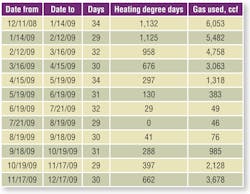
Table 1 presents one year of gas-use data for the office building.
The billing-period and gas-use data came from the customer’s utility bills. “Ccf” stands for 100 cu ft, which is equal to 1 therm or 105 Btu at a nominal higher heating value of 1,000 Btu per cubic foot, typical for utility-supplied natural gas.
Heating degree days came from local weather data. A degree day is calculated by subtracting the mean of the high and low temperature for a day from a base temperature (for heating, usually 65°F).
For example, in Boston on Jan. 25, 2013, the high temperature was 24°F, and the low temperature was 10°F. The mean temperature, then, was 17°F, resulting in 48 heating degree days (HDD) (65 − 17). The number of degree days in any period, such as a month, is the sum of the number of degree days for each day in the period.
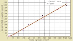
Figure 1 is a plot of gas use against HDD. The solid line is the least mean squares linear regression line. The graph and the regression line lead to the following observations and analysis:
• For this building, like many others, all of the data points are fairly close to the regression line. The factor R2 quantifies how well the line fits the data. R2 ranges from 0, meaning no relationship between the dependent variable (in this case, gas use) and the independent variable (in this case, outdoor temperature as measured by degree days), to 1, meaning perfect correlation.
A lot of scatter in the data (low R2 correlation coefficient) means outdoor temperature is not the main determinant of building energy use. That might be because domestic water heating or other process loads use more energy than space heating does. It also might be because the building uses a lot of energy for reheat or controls do not maintain steady indoor temperature.
It is not unusual for buildings with well-controlled heating systems to have correlation coefficients of 0.96 or 0.98. Buildings with erratic control might show a correlation coefficient of less than 0.80, while buildings with fuel use dominated by domestic water heating or process loads that do not vary with outdoor temperature might show a correlation coefficient of 0.40 or less.
• The equation for the line takes the form of:
y = mx + b
where:
y is gas use in hundreds of cubic feet per month
m is the slope of the line in hundreds of cubic feet per HDD
x is HDD per month
b is the intercept in hundreds of cubic feet per month
The slope, m, provides a measure of actual heating load. By adjusting the units, slope can be expressed in traditional heating-load units of British thermal units per hour per degree Fahrenheit. In this example, the slope of 5.218 ccf per HDD converts to an inferred heating load of 21.74 MBH per degree Fahrenheit of temperature difference, as follows:
5.218 ccf per HDD × 105 Btu per ccf × 1 day ÷ 24 hr = 21.74 MBH per °F
Both heat-loss theory (Q = U × A × ∆T) and fuel-use analysis show fuel use/heat loss is linear with outdoor temperature (as measured by HDD). Therefore, the inferred heating load of 21.74 MBH per degree Fahrenheit can be applied to any indoor/outdoor temperature of interest. For design temperatures of 70°F indoors/0°F outdoors, the inferred design heating load becomes 1,522 MBH.
The intercept, b, represents the amount of gas the building requires at 0 degree days (when outdoor temperature equals the degree-day base temperature: 65°F in most cases). In this building, the intercept is −159.01 ccf per month. With 730 hr in a month, the intercept equates to −22 MBH.
The negative intercept means internally generated heat plus free solar heat gain is more than the heat loss at 65°F (the degree-day base) outdoors. Many well-insulated commercial buildings have a negative intercept.
Buildings with substantial weather-independent loads, or base use, will have a positive intercept, which is the average fuel load to support the base use.
• Comparing the intercept of −22 MBH with the heat-loss rate of 21.74 MBH per degree Fahrenheit (1,522 MBH peak/70°F temperature difference) shows that internally generated heat in the building overcomes 1°F (22 MBH/21.74 MBH per degree Fahrenheit) of indoor-outdoor temperature difference. Expressed another way, the balance point where the building needs neither heating nor cooling is 65°F (degree-day base) minus 1°F, or 64°F. It is not unusual for modern, well-insulated commercial buildings to have an occupied-hours balance point of 35°F to 40°F.
Because it is an accurate measure of actual building heating load, a fuel-use analysis with a high correlation coefficient can be used to size a replacement boiler. While fuel-use analysis is not a substitute for heat-loss calculations, it is a decidedly better measure than British-thermal-units-per-hour-per-square-foot or British-thermal-units-per-hour-per-cubic-foot rules of thumb.
It might be tempting to convert the slope of the fuel-use-analysis regression line to British thermal units per hour. However, that almost certainly would result in an undersized boiler. The reason is that the slope/peak heating load determined from the degree-day analysis is an average over the course of a day. It includes the effects of “free” heat, such as solar gain, and internal heat gains from lights, people, and equipment. A heating system has to be able to heat an empty building at the coldest nighttime hour of the year. Letting the indoor temperature drop several degrees during the coldest hours on the premise the building can catch up later in the day, when the outdoor temperature is higher, might not be acceptable. Experience has shown that increasing the heating load determined from a degree-day slope by 20 percent results in realistic boiler sizing.
Cooling Energy
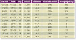
Table 2 presents electricity-use data for the building.
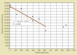
Figure 2 is a plot of electricity use against HDD. Once again, the solid line is the least mean squares linear regression line. The graph and the regression line lead to the following observations and analysis:
• The slope of the cooling-analysis graph is opposite that of the heating-fuel-analysis graph. It is no surprise that HDD go down as outdoor temperature goes up, and cooling load generally goes up as outdoor temperature goes up.
A similar plot could be made with cooling degree days (CDD) on the x-axis. CDD are calculated the same way HDD are (base temperature minus average daily temperature). When electricity use is plotted against CDD, the trend normally is upward to the right—electricity use increasing as CDD and outdoor temperature increase.
The correlation coefficient (R2) of 0.84 for the example building is not as good as the heating-energy correlation coefficient, but is not bad for a cooling analysis. Cooling-energy correlations almost always are lower than heating-energy correlations because factors other than outdoor temperature (e.g., internal heat gains, solar heat gain, humidity) affect cooling load. While solar heat gain and humidity usually rise with outdoor temperature, the relationship is only general. For some buildings, analysis based on cooling degree hours yields a correlation that is quite good. Cooling degree hours are calculated as the difference between hourly temperature and base temperature—no averaging required. Some experimentation might be required to determine the base temperature that produces the best correlation for the building being studied. The workable cooling-degree-hour base temperature might be 55°F, 57°F, 60°F, or even 65°F, depending on the type of building and its use.
• The graph shows a “knee” in the trend at about 600 HDD. There, the trend turns from downward sloping to nearly horizontal. That shows the building has near zero mechanical-cooling load at 600 HDD. A 30-day month produces 600 HDD at an outdoor temperature of 45°F (65°F − [600 ÷ 30]). An analyst might ask why mechanical cooling should have to run at an outdoor temperature of 45°F. The cooling system for this building uses multiple rooftop units. The apparent need to run mechanical cooling at an outdoor temperature of 45°F suggests a look into economizer operation would be justified.
• As with heating energy, the equation for the regression line makes separating mechanical-cooling electricity use from base electricity use possible:
kwh per month = 74,212 kwh per month − 58.191 × HDD per month
The knee in the graph shows no cooling-energy use above 600 HDD per month. Therefore, base electricity use is:
74,212 − (58.191 × 600) = 39,297 kwh per month
Rounding to 40,000 kwh per month, annual base use is:
12 × 40,000 = 480,000 kwh
Annual electricity use from the customer’s utility bills is 610,000 kwh, so cooling accounts for 130,000 kwh. That calculation is consistent with the regression-line slope and number of HDD (2,226) from February through November (the months with fewer than 600 HDD):
58.191 kwh per degree day × 2,226 degree days = 129,533-kwh cooling use
Because the electricity-use line is nearly horizontal above 600 HDD, the data show the building has little or no electric-heating load.
Obtaining Degree-Day Data
Historical temperature data are available from various sources, including the National Weather Service and Weather Underground. The National Weather Service reports the high and low temperatures and number of degree days for each day. Weather Underground does not report degree days, but has data for more locations.
Analysis Tips and Techniques
(1) Analyzing gas and electricity use usually is fairly straightforward because most buildings have monthly metered data. Fuel oil often is delivered in drops or at intervals based on estimated usage. Those intervals could be several months during summer, but only a few weeks during winter. With fuel oil, it sometimes helps to normalize usage and degree-day data to 30-day periods. For example, suppose our office building used 260 gal. of oil over a 22-day period with 847 HDD. The data point for entry into a regression analysis would be:
30 ÷ 22 × 260 = 354.5 gal. of oil
30 ÷ 22 × 847 = 1,155 degree days
Normalizing to a 30-day period works because base use is an important factor in most buildings. Remember that the intercept of the regression line is in units of energy per month (or other selected analysis period).
(2) Because the fuel-use data is energy input, the load determined from a fuel-use analysis is expressed as energy input. Building heat-loss calculations express results as energy output. The difference is boiler or furnace efficiency. While calculated heating loads are divided by boiler efficiency to determine required boiler size, the value of the slope of the regression line is based on energy input and, thus, includes the effect of boiler-efficiency losses.
(3) A high correlation coefficient says only that a system operates consistently and in response to outdoor temperature. It says nothing about equipment or system efficiency. It also says nothing about whether a building is overheated or underheated. Despite such a limitation, fuel-use analysis can provide useful insight. For example, it can sort out the effects of price escalation and weather changes in comparisons of dollar costs from one year to those of another. Also, if the analyst has an idea of what the heating load should be, fuel-use analysis might provide a clue concerning where to look for excessive energy use.
(4) When buildings such as offices and multifamily residences have a substantial base use, that load most often is for domestic water heating. The base use from a regression analysis is the average over the course of a month, including over night, when there is little or no domestic-hot-water use. Unless a system has a lot of hot-water storage, a boiler needs to deliver much more heat than the average “base” load on a call for domestic water heating. Few phenomena in nature have a peak-to-average ratio (crest factor) greater than 3:1 (a sine wave, which is typical of many phenomena, has a peak-to-average ratio of √2:1, or 1.414:1). Therefore, when sizing a replacement boiler based on energy-use data, a factor of three times the base-use intercept often is a good allowance for domestic-water-heating capacity.
(5) Table 2 contains a column labeled “Hours use of demand.” This is the kilowatt-hours in a period divided by the peak demand (kilowatts) for the period. It represents the demand needed for the system to operate continuously for an entire billing period (usually a month) to produce billed kilowatt-hour consumption.
Hours use of demand is not used in degree-day analysis, but provides useful insight into electricity use. There are 730 hr in a month, so for bills rendered monthly, hours use of demand has to be between 1 and 730. Typical office buildings in the northeast United States range from 300 to 350 hr use of demand. Higher hours use of demand, especially during winter, suggests an electrically heated building. Otherwise, hours use of demand over 400 or 450 raises a question of whether unnecessary loads operate during unoccupied hours. An oversized cooling system with few steps of control might increase demand enough to push hours use down to 100 or less. That low an hours use of demand suggests looking into some type of control to reduce peak demand.
Motor starting inrush current often is not a reason for excessive demand. Motor starting power factor typically is in the range of 20 percent (compared with 85 percent to 90 percent for an operating motor). Most of the high current draw during motor start-up goes to magnetizing current to develop torque. Magnetizing current does not develop real power that the kilowatt-hour meter measures. More importantly, metered demand is the highest number of kilowatt-hours measured during a demand-period window, not a momentary reading. Sometimes, the demand window is a half-hour; sometimes, it is 15 min; sometimes, it is the highest three consecutive 5-min periods. Motor starting current draw lasts only a few seconds, so even if a motor draws a lot of power during start-up, that high power draw is divided over the demand-period window to determine peak demand. Averaged over a 15-min demand window, starting a motor does not “spike” demand. Running it for several minutes, however, contributes to demand.
Summary
The ability to analyze utility bills is another skill in an engineer’s arsenal of tools to understand HVAC energy use and find ways to use energy effectively in buildings. This article described a concept and how to apply it.
This file type includes high resolution graphics and schematics when applicable.
A longtime member of HPAC Engineering’s Editorial Advisory Board, Kenneth M. Elovitz is an engineer and the in-house counsel for Energy Economics Inc. His knowledge of and experience with HVAC, electrical, and life-safety systems allow him to understand system function and performance, including interactions among disciplines. He is an adjunct instructor in the Architectural Engineering program at Worcester Polytechnic Institute.
Did you find this article useful? Send comments and suggestions to Executive Editor Scott Arnold at [email protected].
About the Author
KENNETH M. ELOVITZ
Engineer and In-House Counsel
A longtime member of HPAC Engineering’s Editorial Advisory Board, Kenneth M. Elovitz is an engineer and the in-house counsel for Energy Economics Inc. His knowledge of and experience with HVAC, electrical, and life-safety systems allows him to understand system function and performance, including interactions among disciplines. He is an adjunct instructor in the Architectural Engineering program at Worcester Polytechnic Institute.