Data logging is great for finding equipment-scheduling opportunities in buildings, but its use does not end there. This article discusses applications related to economizers, cycling fans, and simultaneous heating and cooling, boiler lockouts, and supply-air resets.
Economizers
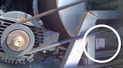
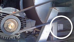
In a field survey of 500 economizers, 64 percent were found to have failed.¹ How can you tell if an economizer has failed? With data loggers. You will need three: one to measure outside-air temperature, one to measure return-air temperature, and one to measure mixed-air temperature. Or, you could use a single four-channel data logger with three temperature sensors. Getting a good reading of mixed-air temperature can be difficult because of air striation. Just before the inlet to a supply fan (Photo A) or just after filters is a good spot to place a sensor.
The temperature of mixed air follows a simple equation, related to the percentage of outside air being used:
MAT = OAT × x + RAT × (1 − x)
where:
MAT = mixed-air temperature
OAT = outside-air temperature
x = percentage of outside air
RAT = return-air temperature
You can solve this equation for x, yielding the relationship:
x = (MAT − RAT) ÷ (OAT − RAT)
Using data loggers, you can learn what the mixed-, return-, and outside-air temperatures are and determine if an economizer is working.
Unfortunately, the outside-air temperature may be rather close to the return-air temperature, making the equation go to infinity because the denominator is zero. This can be overcome with some simple graphs.
Make a scatter plot of your logged data, with the x-axis OAT − RAT and the y-axis MAT − RAT. Discard the data recorded when the unit was turned off.
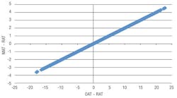
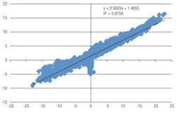
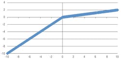
If the unit is not equipped with an economizer, you may see something resembling Figure 1. Figure 1 was created using measured outside-air and return-air temperature; for mixed-air temperature, a theoretical model based on dampers letting in 20-percent outside air was used. Note that the slope of the line is 0.2. The economizer will be between these positions when outside-air temperature is less than 55°F (left side of the graph). Using real-world data, you may get a graph more closely resembling Figure 2. Note that the slope is closer to 0.57, indicating the air handler is stuck at 57-percent outside air.
If the unit is equipped with an economizer, you may see something like Figure 3. Note the difference in slopes. On the left side of the graph, the slope is 1, indicating the unit is at 100-percent outside air. On the right, the slope is 0.2, indicating the economizer dampers are at a minimum.
Now that you can tell whether or not your economizer is working, you can calculate savings.
A building’s cooling or heating system takes mixed air and cools or heats it to the desired supply-air temperature. The energy use is equal to:
1.08 × cfm × ∆T = energy
where:
1.08 = constant related to the density and specific heat of air at sea level. (Note: A different constant is used for higher altitudes.) This makes the equation produce a result in British thermal units.
cfm = flow rate across the fan, which can be found in building design documents
∆T = difference between mixed-air temperature and supply-air temperature
Knowing energy use, you can download typical-meteorological-year (TMY) data to get hourly weather patterns for your site and to calculate mixed-air temperature with and without an economizer for every hour of the year. Using the airflow rate of your system, you then can calculate the energy savings from installing or repairing an economizer. (Note: The above calculation does not account for latent cooling. In the San Francisco Bay Area, a factor of 0.25 to 0.3 is conservative as an adder to account for dehumidification.)
Cycling Fans
With data loggers, you can accurately forecast energy savings resulting from the installation of variable-frequency drives (VFDs) on pumps and fans.
VFDs take advantage of the affinity laws. In this case, you need only one:
(P1 ÷ P2) = (RPM1 ÷ RPM2)³
This can be rewritten as:
P1 = P2 × (RPM1 ÷ RPM2)³
where:
P1 = fan or pump power at a slow (or fast) speed
P2 = fan or pump power at a fast (or slow) speed
RPM1 = the slow (or fast) speed
RPM2 = the fast (or slow) speed
(Note: The affinity laws are a bit idealized compared with results in the field. If you are installing a VFD on a pump or fan with high static head, you are better off using an exponent of 2.2, as opposed to 3. If the pump or fan has relatively low static head, an exponent of 2.7 is recommended.)
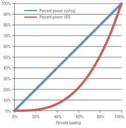
The important thing to note about the above equation is that as VFD speed decreases, power decreases like the cube. So, if you cut the speed in half, you end up using only 12.5 percent of the power. To illustrate, assume P2 is the power of the fan when operating at 60 hertz without a VFD. Then, we see:
P1 = 100% × (30 ÷ 60)³ = 12.5%
Imagine a 100-kw fan cycling half of the time. Over the course of an hour, the fan would consume 50 kwh of energy. If a VFD were installed and turned down to 50-percent speed, the fan would consume only 12.5 kwh of energy over the course of an hour, a savings of 37.5 kwh (Figure 4).
To predict fan speed, which will change throughout the year based on weather conditions, we need to measure the cycle rate of the fan and regress it against weather.
Connect a current transformer to your data logger, and measure the current going into the fan motor. To calculate cycle rate accurately, use 1- or 2-min interval data. Use another data logger to measure outside-air conditions, or download National Oceanic and Atmospheric Administration data. Now, calculate your cycle rate for each hour, and compare that to your outside-air-temperature data. Keep in mind that cooling towers track wet-bulb temperature, while evaporator fans are likely to track dry-bulb temperature.
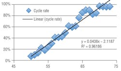
The result should be a graph similar to Figure 5. Note that the fan starts coming on at 49°F and is at 100 percent by 72°F. Between these two temperatures, the cycle rate follows the equation:
Cycle rate = 0.0438 × OAT − 2.1187
If the fan is cycling at 50 percent, the load your system is experiencing is 50 percent of the design capacity. Again, energy use follows the equation:
1.08 × cfm × ∆T = energy
If we reduce flow rate across the fan by half, we get half the energy transfer, the effect of the fan cycling off half of the time. VFD speed, then, is equal to fan cycle rate. (Note: There is a built-in assumption that a reduction in fan speed will not change delta-T across the coil. In fact, a reduction in fan speed probably will lead to a slightly higher delta-T, meaning speed could be reduced even further. Thus, savings estimates will be slightly conservative.)
Now, you are ready to calculate savings. Create a spreadsheet. In the first column, enter the annual weather data. In the next column, calculate cycle rate based on the weather (cap the cycle rate so it does not go lower than zero or higher than 100 percent). The next column should be baseline energy use: the cycle rate times the fan power draw (in kilowatts, measured with a power meter to account for power factor and voltage). In the final column, use the fan affinity law presented above to calculate the energy use of the fan with a VFD.
Subtract the last two columns, and you have calculated energy savings. (Make sure to account for scheduling.)
Simultaneous Heating/Cooling, Boiler Lockouts, Supply-Air Resets
Supply-air resets can be a great way to reduce energy use in a variable-air-volume (VAV) system. To calculate savings from supply-air resets, one must log:
• The temperature of the air coming out of the air handler.
• The temperature of the air outside (dry bulb).
• Some of the hottest zones in the building or the zones with the coolest air coming out of the registers (likely, on the south or west side of the building).
Unless you have been with the building since construction or you have a good controls system, the first thing you should do is check supply-air temperature across a range of outside-air temperatures to make sure you are not performing a supply-air reset already. If supply-air temperature always is between 52°F and 58°F, then the compressor probably is cycling. Do a regression of supply-air temperature based on outside-air temperature to check. If your line basically is flat (e.g., always 55°F or 58°F), then you do not have a supply-air reset. If your line slopes significantly—supply-air temperature is 55°F when outside-air temperature is above 75°F and 65°F when outside-air temperature is below 40°F—then you probably do have a supply-air reset.
The simplest way to control supply-air reset is based on outside-air temperature. This is how we will calculate savings. The equation we will rely on is:
1.08 × cfm × ∆T = Btu
where:
1.08 = constant based on altitude
To calculate flow rate, you need to know the maximum airflow, which occurs during the cooling design day. This information can be found in air-handler cut sheets. You also need to know the outside-air temperature at which the VAV boxes close to minimum position and what that minimum position is.
Suppose you know the following about your building:
• The design day is 100°F.
• The maximum flow rate through the air handler is 50,000 cfm.
• The VAV boxes close to a minimum position when outside-air temperature is 45°F.
• The minimum position is 25 percent.
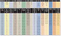
You now are prepared to calculate flow rate based on outside-air temperature. When the outside-air temperature is 100°F, the flow rate is 50,000 cfm; when the outside-air temperature is 45°F, the flow rate is 12,500 cfm (Table 1). Between those two points, flow rate follows a linear ramp:
y = mx + b
where:
y = flow rate
m = slope
b = y-intercept
The slope is equal to the change in flow rate over the change in outside-air temperature:
m = (50,000 − 12,500) ÷ (100 − 45) = 681.82
The y-intercept can be found by solving for a known point—namely, 100°F outside-air temperature—and using the slope above:
50,000 = 681.82 × 100 + b → b = 50,000 − 68,182 = -18,182
To ensure the equation works, let’s plug in 45°F outside air:
cfm = 681.82 × 45 − 18,182 = 12,499.99 ≈ 12,500
Now, we can calculate flow rate based on outside-air temperature using the equation for flow rate we developed.
Once we know the delta-T, we can finish calculating energy savings. In this case, there are two delta-Ts: from the mixed air to the supply air and from the supply air to the discharge air. The former indicates cooling energy use, while the latter indicates reheat use.
To calculate cooling energy use, we need to know the mixed-air temperature across a range of outside-air temperatures. If you do not have an economizer and use a constant 20-percent outside air, this is simple:
MAT = OAT × 0.2 + RAT × 0.8
Usually, you can assume return-air temperature is roughly equal to or one or two degrees higher than space temperature. If you assume a flat 72°F year-round, you will be fairly accurate.
For outside-air temperature, you can download a TMY file for every hour of the year for your building.
Even if you have an economizer, calculating mixed-air temperature is relatively easy. Assuming a supply-air-temperature setpoint of 55°F and an outside-air temperature below 55°F, mixed-air temperature will be 55°F. If outside-air temperature is greater than 55°F, but less than, say, 70°F, mixed-air temperature will be the same as outside-air temperature. If outside-air temperature is above 70°F, mixed-air temperature will follow the equation above.
For cooling energy:
1.08 × cfm × (MAT − SAT)
For reheat energy, log the discharge-air temperature at a few VAV boxes, as well as outside-air temperature. Next, create a graph with discharge-air temperature on the y-axis and outside-air temperature on the x-axis. Add a trend line, and you can see what discharge-air temperature should be across a range of outside-air temperatures. (Do not forget to eliminate data for unoccupied times.)
Now, you are ready to calculate energy use. In the base case, you have energy use with a static supply-air setpoint. In the retrofit case, you have a supply-air reset. For boiler resets, lock out your boiler (and heating water pumps) when outside-air temperature exceeds 70°F (this may vary a bit, based on region and building, but is a good starting point). Calculating savings from a boiler lockout is simple: Heating energy use above 70°F goes to zero, as does energy use for pumps.
You also can combine a supply-air reset with a boiler lockout. Table 2 shows savings at a range of temperatures. To calculate annual savings, download a TMY weather file, and perform an analysis for each hour of the year using the methods outlined here. Heating energy savings should be divided by the efficiency of your boiler; cooling energy savings should be divided by your unit’s coefficient of performance. Lastly, do not forget to take scheduling into account, and do not forget pump savings from your boiler lockout.
Reference
1) Hart, R., Callahan, J., Anderson, K., & Johanning, P. (2011). Unitary HVAC premium ventilation upgrade. Paper presented at 2011 ASHRAE Winter Conference, Las Vegas. Available at http://www.peci.org/sites/default/files/unitary_hvac_premium_ventilation_upgrade.pdf
Brenden Millstein is co-founder and chief executive officer of Carbon Lighthouse, an engineering company dedicated to making carbon neutrality profitable for organizations. Previously, he worked for the New York State Energy Research & Development Authority and, before that, as a research fellow at Lawrence Berkeley National Laboratory. To date, he has been involved in more than 400 energy-efficiency and demand-response projects in California, Oregon, and New York. He has a bachelor’s degree in physics from Harvard University and master’s degrees in renewable-energy engineering and business administration from Stanford University.
Did you find this article useful? Send comments and suggestions to Executive Editor Scott Arnold at [email protected].
